SPEED DISTRIBUTIONS
A few basic statistical concepts are introduced in this chapter to help with an understanding of speed terms and principles.
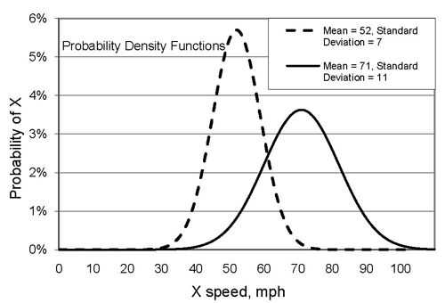
Speeds are selected by the driver. Different drivers select different speeds, dependent upon many variables (vehicle limitations, roadway conditions, driver ability, etc.). No single speed value can accurately represent all the speeds at a particular location. A speed distribution (see definition in chapter 2) provides that information. Operating speeds have been found to be normally distributed (sometimes called a "bell-shaped curve"). This is fortunate since using that premise (probability is normally distributed) allows for some straightforward calculations. Even though a variable (e.g., speed, height) may be normally distributed, properties of the distribution may vary. Two different normal probability density functions are shown in figure 6. The vertical axis indicates the probability that the variable will take on the corresponding value on the horizontal axis. The speed distribution provides useful information but it is not a convenient way to describe speeds.
Figure 6. Normal probability distributions.
The unique properties of the normal probability distribution allow it to be conveniently described with just two characteristics, mean and standard deviation. These two characteristics also have practical importance for traffic speeds. Figure 7 includes plots of two different normal speed distributions. These distributions have the same mean but different standard deviations.
Figure 7. Examples of two normal probability distributions, operating speeds, same mean, different standard deviations.
For reasons stated elsewhere in this Informational Guide, the 85th percentile speed is a frequently used characteristic. The mean speed plus one standard deviation approximates the 85th percentile speed for a normally distributed sample of speeds. For an observed sample of speed data, determining the 85th percentile value is fairly easy, either manually (for relatively small samples) or a spreadsheet. To get a graphical sense of the 85th percentile speed, the cumulative distribution function can be plotted. An example is included as figure 8. To find the values associated with any Nth percentile (e.g., 25th, 60th or 85th percentile) level, find that percentile level on the vertical axis. Then move horizontally until the line representing the cumulative distribution function is intersected, project a line from that point down to the intersection with the horizontal axis. The value on the horizontal axis is associated with the Nth percentile. For the figure 8 example, the 85th percentile speed is 59 mph.
SPEED PROFILES
Speed profiles are a graphical representation of speed features plotted by location. Figure 9 is an example. Speed profiles are useful in studies and evaluations. The contents of speed profiles vary but features that are commonly included are the designated design speed, operating speed and posted speed limit; inferred design speed can be displayed as well.
Figure 8. Example cumulative distribution function, operating speeds.
Figure 9. Example speed profile.


