
3.1 Light and Vision
Many factors influence our ability to see an object while driving. These include the contrast of the object, both photometric and color (i.e., the difference between the object and its background); the driver's adaptation level (impacted by the brightness of the road and surrounds, how much glare is present from approaching vehicles and luminaires, etc.), and how long the driver has to view a hazard. Understanding these factors is vitally important to developing an effective design for roadway and street lighting.
3.1.1 Structure of the Eye
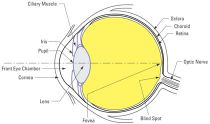
Figure 3 - Fundamental Structure of the Human Eye
The retina contains two types of photoreceptors, rods and cones. Rods, which are most numerous in the retina, are more sensitive and function at a lower light level than the cones. Rods are also not sensitive to color. Cones are sensitive to color and are divided into red (64 percent), green (32 percent), and blue (2 percent) cones. They are concentrated in the macula of the eye with most being in the center of that region, the fovea, which contains only cones.
In the 1990s a third type of photoreceptor was discovered and named "intrinsically photosensitive Retinal Ganglion Cells" (ipRGCs). More research is being conducted into the function of these photoreceptors as they relate to controlling adaptation, restriction of the pupil, and circadian rhythms. Their application to roadway lighting at this time is unclear.
Adaptation of the eye occurs in the retina, as the eye adjusts to the varying brightness of a scene caused by the overhead lighting system, approaching vehicle headlights, and ambient lighting conditions. States of adaptation include:
- Scotopic Vision – Vision by the normal human eye, when only the rods of the retina are being used, where the adaptation luminance at the eye is 0.001 cd/m2 or lower. At this state of adaptation there is no sensation of color.
- Mesopic Vision – when both the rods and cones are active, at varying percentages based on based on conditions, where the adaptation luminance at the eye is between 0.001 cd/m2 and 3.0 cd/m2. At this state of adaptation the eye is sensitive to color (more "blue" at the lower end of the adaptation range and more "red" at the higher).
- Photopic Vision – when predominantly cones are active and normal color vision is possible, where the adaptation luminance at the eye is 3.0 cd/m2 and above.
3.1.2 Spectral Properties
Visible light is a limited range of electromagnetic radiation. Within this range, different wavelengths are seen as different colors. As Figure 4 demonstrates, radiation with a shorter wavelength on the visible spectrum is perceived as more "blue" in color, while radiation with a longer wavelength is perceived as more "red."
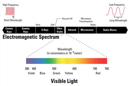
Figure 4 - Electromagnetic Spectrum and Visible Spectrum
The eye has varying sensitivity to different wavelengths within the visible spectrum depending on the state of adaptation.
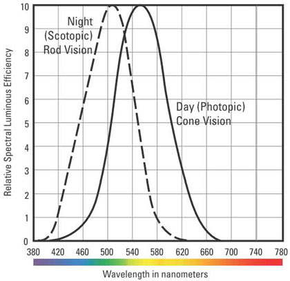
Figure 5 - Eye Sensitivity Curves
The solid curve in Figure 5 is referred to as the V Lambda V(l) curve. This curve represents the spectral efficiency of a source when the eye is using photopic vision. Sources with wavelengths in the more "yellow" range, such as high pressure sodium, would be rated at a higher power value (lumen) than a source with the same amount of more "blue" content, such as metal halide of higher Correlated Color Temperature (CCT) LED sources.
The dashed curve represents the eye response when using scotopic vision. This shows that at very low light levels sources with more "blue" content would be allocated a higher lumen value.
3.2 Fundamentals of Visibility
3.2.1 Contrast
Objects are seen by "contrast," which is basically the visible difference between an object and its background. From a luminance perspective, an object that is darker than its background will be seen by "negative" contrast, and an object that is sufficiently brighter than its background will be seen by "positive" contrast. In Figure 6, the upright object shown in the upper frames is in negative contrast (a darker object silhouetted against a brighter background), and in the lower frames it is in positive contrast (brighter object against darker background). It is also worth noting that contrast may vary within the object itself. The upper right frame shows the bottom portion of the object in negative contrast, and the upper portion in positive contrast. The value of contrast also changes along its length.
The formula for calculating contrast (Weber contrast) is:
| Contrast = | LObject – LBackground _______________________________________ LBackground |
LObject = Luminance of the object
LBackground = Luminance of the background
If we use the luminance values shown in the upper portion of the figure we can calculate that the lower portion of the cylinder, where the roadway is the background, has a contrast of (1-22)/22 = -0.95, with the negative value denoting that it is negative contrast.
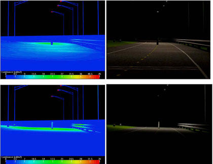
Figure 6 - Luminance Contrast (negative contrast above and positive below)
This contrast value is the luminance contrast of the object. How much contrast you need to see an object depends on a number of things, including the size of the object, how long you look at it, your age, and your adaptation luminance (determined by the luminance of the road, glare from lights, approaching headlights, and ambient lighting levels). This is called the threshold contrast and is based on the probability of detection of an object 50 percent of the time (Adrian, 1989) (12). The purpose of a roadway lighting system is to produce actual contrast of an object on the road greater than the threshold contrast required by the driver for detecting it. Studies (Blackwell) (13) suggest that good visibility of objects can be achieved if the actual contrast is 3 to 4 times the required threshold contrast. Obtaining this contrast is primarily a function of the lighting placement and optical characteristics.
Applying contrast metrics to roadway lighting, however, is situational and depends on many variables. Designers should nevertheless be aware of the key elements under their control:
- Control/reduce the glare generated by the roadway lighting system.
- If possible, reduction of glare from approaching headlights by median widths and treatments will increase visibility.
Color also provides additive contrast benefits. As shown in Figure 7, the visibility of objects and pedestrians can be improved by color contrast. This is dependent upon the color of the object or clothing as well as the color rendering ability of the source used for roadway lighting. In looking at the pedestrian's red shirt or the approaching red vehicle in the left frame of Figure 7, we can tell that color contrast provides additional visibility. This effect is quite variable, however, so it is not quantified for roadway lighting.
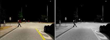
Figure 7 - Effect of Color Contrast
3.2.2 Glare
Non-uniformities in the visual field, particularly those caused by bright sources, affect the adaptation level of the eye. Because these sources tend to fluctuate as the driver proceeds, the adaptation level is constantly changing ("transient adaptation"). Roadway lighting thus aids the eye in adapting to an increased level of luminance than can be provided by headlights alone. Bright sources create other effects, collectively termed "glare," which should be avoided as much as is practical.
Disability Glare
Light rays passing through the eye are slightly scattered, primarily because of diffusion in the lens and the vitreous humor that fills the anterior chamber of the eye. When a light source of high intensity is present in the field of view, this scattering tends to superimpose a luminous haze over the retina. The effect is similar to looking at the scene through a luminous veil. The luminance of this "veil" is added to both the task and background luminance, thus having the effect of reducing contrast. The effect is termed "disability glare" or "veiling luminance," and it may be numerically evaluated by expressing the luminance of the equivalent luminous veil. A well-known example of this is trying to see beyond oncoming headlights at night. Because of contrast reduction by disability glare, visibility is decreased. Increasing luminance will counteract this effect by reducing the eye's contrast sensitivity. A well designed roadway lighting system will minimize glare by employing luminaires that have proper optical design (e.g., cutoff or full-cutoff). Disability glare should be limited to the recommended veiling luminance ratios included in the AASHTO (26) and IES(28) recommendations.
Disability glare is one of the most important elements to control in a lighting system. It affects your ability to adequately see, particularly for older drivers.
Discomfort Glare
Discomfort glare is a further result of overly bright light sources in the field of view, and causes a sense of pain or annoyance. While its exact cause is not known, it may result from pain in the muscles that cause closing of the pupil. Disability glare and discomfort glare normally accompany one another, and beneficial luminaire light control that reduces one form of glare is likely to reduce the other. Discomfort glare, which can cause effects from an increased blink rate to tears and pain, does not reduce visibility. It is also generally accepted that reducing disability glare will reduce discomfort glare. It is possible, however, to reduce discomfort glare and increase disability glare. North American roadway lighting standards do not specify numerical limits for discomfort glare. Methods exist to quantify discomfort glare for roadway lighting, but are mostly subjective. Also, no instrument has been developed for the measurement of discomfort glare. The Commission Internationale de l'Eclairage (International Commission on Illumination - CIE) uses a "Glaremark System," which is a graphical method using a scale of 1 to 10 to rate lighting systems. However, there is no current practical use or application of this method.
Nuisance Glare
The presence of extraneous light in the field of view may cause a nuisance or distraction to the driver, independent of the effects of disability and discomfort. Bright light sources tend to cause distraction, and the eye may be drawn to them. Lighting that is used for advertising, for example, may cause visual clutter and add complexity to the scene, making the driving task more challenging. There is no defined method or measurement system for assessing nuisance glare.
3.2.3 Perception-Reaction Time
Many components make up perception-reaction time. A motorist, in order to stop or avoid a hazard or person on a roadway, must first detect the object's presence, recognize or otherwise assess the object, then react to that determination. The mechanical operation of braking/steering mechanisms, as well as road/tire/vehicle performance conditions, also factor into perception-reaction time.
From a reaction time perspective, key elements include whether a situation is expected, cognitive load and distractions, personal physical response attributes, age, and other factors, Green (22) classified reaction times, adding an additional condition of "surprise", in the following way:
- Expected - The driver is alert and aware of the good possibility that braking will be necessary. This is the absolute best reaction time possible. The best estimate is 0.7 seconds (AASHTO Green Book (14) states it as approx. 0.6 seconds). Of this, 0.5 is perception and 0.2 is movement, the time required to release the accelerator and to depress the brake pedal.
- Unexpected - The driver detects a common road signal such as a brake from the car ahead or from a traffic signal. Reaction time is somewhat slower, about 1.25 seconds (AASHTO Green Book (14) states it is approx. 35% longer than the expected condition). This is due to the increase in perception time to over a second with movement time still about 0.2 second.
- Surprise - The driver encounters a very unusual circumstance, such as a pedestrian or another car crossing the road in the near distance. T here is extra time needed to interpret the event and to decide upon response. Reaction time depends to some extent on the distance to the obstacle and whether it is approaching from the side and is first seen in peripheral vision. The best estimate is 1.5 seconds for side incursions and perhaps a few tenths of a second faster for straight-ahead obstacles. Perception time is 1.2 seconds while movement time lengthens to 0.3 second."
For example a person traveling at 55mph is moving at approximately 80 ft/sec. The distance traveled during reaction time alone can be anywhere from 40' to 120'. When this is added to the distance covered during actual stopping, the total can be quite significant.
The AASHTO Policy on Geometric Design of Streets and Highways (14) include a method for determining stopping distance based on a number of factors including reaction time. Figure 8 shows examples of estimated Safe Stopping Sight Distance (SSSD) based on that AASHTO method with modifiers showing the impact of grades.
| Metric | U.S. Customary | ||||||||||||
|---|---|---|---|---|---|---|---|---|---|---|---|---|---|
| Design | Stopping Sight Distance (m) | Design | Stopping Sight Distance (m) | ||||||||||
| Speed | Downgrades | Upgrades | Speed | Downgrades | Upgrades | ||||||||
| (km/h) | 3% | 6% | 9% | 3% | 6% | 9% | (mph) | 3% | 6% | 9% | 3% | 6% | 9% |
| 20 | 20 | 20 | 20 | 19 | 18 | 18 | 15 | 80 | 82 | 85 | 75 | 74 | 73 |
| 30 | 32 | 35 | 35 | 31 | 30 | 29 | 20 | 116 | 120 | 126 | 109 | 107 | 104 |
| 40 | 50 | 50 | 53 | 45 | 44 | 43 | 25 | 158 | 165 | 173 | 147 | 143 | 140 |
| 50 | 66 | 70 | 74 | 61 | 59 | 58 | 30 | 205 | 215 | 227 | 200 | 184 | 179 |
| 60 | 87 | 92 | 97 | 80 | 77 | 75 | 35 | 257 | 271 | 287 | 237 | 229 | 222 |
| 70 | 110 | 116 | 124 | 100 | 97 | 93 | 40 | 315 | 333 | 354 | 289 | 278 | 269 |
| 80 | 136 | 144 | 154 | 123 | 118 | 114 | 45 | 378 | 400 | 427 | 344 | 331 | 320 |
| 90 | 164 | 174 | 187 | 148 | 141 | 136 | 50 | 446 | 474 | 507 | 405 | 388 | 375 |
| 100 | 194 | 207 | 223 | 174 | 167 | 160 | 55 | 520 | 553 | 593 | 469 | 450 | 433 |
| 110 | 227 | 243 | 262 | 203 | 194 | 186 | 60 | 598 | 638 | 686 | 538 | 515 | 495 |
| 120 | 263 | 281 | 304 | 234 | 223 | 214 | 65 | 682 | 728 | 785 | 612 | 584 | 561 |
| 130 | 302 | 323 | 350 | 267 | 254 | 243 | 70 | 771 | 825 | 891 | 690 | 658 | 631 |
| 75 | 866 | 927 | 1003 | 772 | 736 | 704 | |||||||
| 80 | 965 | 1035 | 1121 | 859 | 817 | 782 | |||||||
Figure 8 - Examples of AASHTO Calculated Safe Stopping Sight Distance with Variation Due to Grade
Although stopping distances are not applied to roadway lighting, with the exception of tunnel lighting systems, the distances shown demonstrate one of the benefits of roadway lighting. If we assume most low beam vehicle headlights have an effectiveness of approximately 300' in front of the vehicle (Green, 2008) (23), speeds of 40 mph and above have stopping distances greater than that distance. In order for a driver to detect a pedestrian or road hazard in time to stop at higher speeds, the roadway lighting system needs to provide that necessary visibility.
At speeds above 40mph roadway lighting provides visibility of objects beyond the effective range of headlights
3.2.4 Spectral Effect Models
As discussed in the Light and Vision section of this handbook, the color of light (wavelength) produces different responses in the eye depending on its state of adaptation. There were established response curves for adaptation in the photopic and scotopic states, but none established for the mesopic state which would change depending on the adaptation luminance. However, models have been developed in recent years suggesting modifying factors which can be applied to adjust the calculated photopic luminance value to the expected mesopic luminance based on the source spectral distribution (Scotopic/Photopic -S/P- ratio). Ongoing discussion and further research is being performed in this area so these models are provided as information.
MOVE – Mesopic Optimisation of Visual Efficiency
The MOVE method was developed from tests conducted at the TNO (Netherlands), University of Veszprem (Hungary), Darmstadt University of Technology (Germany), City University (UK), and Helsinki University of Technology (Finland). From this research modifiers were developed for adaptation luminance and source S/P ratios of various values. Those modifiers are shown in Figure 9.
As an example, a high pressure sodium roadway fixture might have an S/P ratio of around 0.6; if lamped with pulse start metal halide it might be around 1.4; and with an LED roadway fixture it may be 2.0. So using the MOVE multipliers, if we assume the adaptation luminance is 1 cd/m2 the mesopic luminance for the HPS luminaire would be approximately 0.93 cd/m2, the MH luminaire would be approximately 1.06 cd/m2, and the LED luminaire would be approximately 1.15 cd/m2.
| S/P | 0.01 | 0.03 | 0.1 | 0.3 | 1 | 3 | 10 |
|---|---|---|---|---|---|---|---|
| 0.25 | 0.0025 | 0.0075 | 0.064 | 0.2331 | 0.8735 | 2.8108 | 9.9095 |
| 0.35 | 0.0035 | 0.0133 | 0.0698 | 0.243 | 0.8914 | 2.8372 | 9.922 |
| 0.45 | 0.0045 | 0.0172 | 0.0751 | 0.2525 | 0.909 | 2.8632 | 9.9344 |
| 0.55 | 0.0055 | 0.0201 | 0.0801 | 0.2616 | 0.9262 | 2.8888 | 9.9466 |
| 0.65 | 0.0065 | 0.0226 | 0.0848 | 0.2706 | 0.9431 | 2.9141 | 9.9587 |
| 0.75 | 0.0075 | 0.0249 | 0.0894 | 0.2792 | 0.9597 | 2.9391 | 9.9706 |
| 0.85 | 0.0085 | 0.027 | 0.0937 | 0.2877 | 0.976 | 2.9637 | 9.9825 |
| 0.95 | 0.0095 | 0.029 | 0.0979 | 0.2959 | 0.9921 | 2.988 | 9.9942 |
| 1.05 | 0.0105 | 0.0309 | 0.0102 | 0.304 | 1.079 | 3.012 | 10.0058 |
| 1.115 | 1.0114 | 0.0328 | 0.106 | 0.3119 | 1.0234 | 3.0356 | 10.0173 |
| 1.25 | 0.0122 | 0.0345 | 0.1099 | 0.3197 | 1.0387 | 3.059 | 10.0286 |
| 1.35 | 0.013 | 0.0362 | 0.1136 | 0.3273 | 1.0538 | 3.0822 | 10.0399 |
| 1.45 | 0.0138 | 0.0378 | 0.1173 | 0.3348 | 1.0686 | 3.105 | 10.051 |
| 1.55 | 0.0146 | 0.0394 | 0.1209 | 0.3421 | 1.0833 | 3.1276 | 10.0621 |
| 1.65 | 0.0153 | 0.041 | 0.1245 | 0.3493 | 1.0978 | 3.1499 | 10.073 |
| 1.75 | 0.016 | 0.0425 | 0.128 | 0.3565 | 1.1121 | 3.172 | 10.0838 |
| 1.85 | 0.0167 | 0.044 | 0.1314 | 0.3635 | 1.1262 | 3.1939 | 10.0945 |
| 1.95 | 0.0174 | 0.0455 | 0.1348 | 0.3704 | 1.1401 | 3.2155 | 10.1051 |
| 2.05 | 0.018 | 0.0469 | 0.1381 | 0.3772 | 1.539 | 3.2368 | 10.1156 |
| 2.15 | 0.0187 | 0.0483 | 0.1413 | 0.384 | 1.1675 | 3.258 | 10.126 |
| 2.25 | 0.0193 | 0.0497 | 0.1445 | 0.3906 | 1.181 | 3.2789 | 10.1363 |
| 2.35 | 0.0199 | 0.0511 | 0.1477 | 0.3972 | 1.1943 | 3.2997 | 10.1466 |
| 2.45 | 0.0205 | 0.0524 | 0.1509 | 0.4037 | 1.2075 | 3.3202 | 10.1567 |
| 2.55 | 0.0211 | 0.0538 | 0.1539 | 0.4101 | 1.2205 | 3.3405 | 10.1667 |
| 2.65 | 0.0217 | 0.0551 | 0.157 | 0.4165 | 1.2334 | 3.3606 | 10.1766 |
| 2.75 | 0.0223 | 0.0564 | 0.1600 | 0.4228 | 1.2462 | 3.3806 | 10.1865 |
Figure 9 - Modifiers from MOVE Model
Rea et al - Unified System of Photometry
The unified system of photometry was developed by conducting a field study on a test road where subjects were asked to identify the orientation of various size Landolt rings displayed on small targets in the center of the roadway. Their reaction time was measured, as well as their subjective impressions of visibility. These results were then compared with various models for photometry in the mesopic region. The comparative models used are shown in Figure 10.
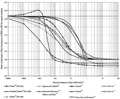
Figure 10 - Figure from Rea's A proposed system of photometry - Lighting Res. Tech. 36.2 (2004 pp. 85-111)
Rea's research also included a condensed summary of other research and models (shown in Figure 11) to allow for easy comparison'
| Author | Method | Stimuli | Size of Target | Position | Adaptation Light Levels | Model to obtain mesopicluminance |
|---|---|---|---|---|---|---|
| Palmer19:30 | Heterochromatic brightness matching: monocular Maxwellian view of a 5°, 15° and 45° horizontally bisected circular field; 21° white surround | Nearly monochromatic to broad spectrum sources, covering the spectrum, reference tungsten light 2042 K | 5°, 15° and 45° | foveal | 0.000316 to 0.316 cd/m2 in 0.5 log unit steps | Empirical, non-linear average of photopic and scotopic luminance, with a variable M that depends on visual size. Revised model using the same variables as the original |
| Ikeda and Shimozono 32 Nakano and Ikeda 33 | Heterochromatic brightness matching: two-channel Maxwellian view of a 10° bipartie field | Four pairs of monochromatic combinations (460, 630; 490, 610; 470, 580; 500, 570mm) at different proportions from all of one to all of the other, white reference | 10° | foveal | 0.01, 0.1, 1, 10, 100Td | Set of equations, with parameters defined for a 7mm pupil and 10° field of view |
| Sagawa and Takeichi 20.21 | Heterchromatic brightness matching; two channel Maxwellian view of a 10 bipartite field; 3mm artificial pupil | Monochromatic, 400 to 700 nm in 10 nm steps | 10° | foveal | 0.01 to 100Td in 0.5 log unit steps | Graphic determination of mesopic luminance; use brightness luminous efficiency functions normalized at 570nm. One coefficient method for broad spectrum sources, two coefficients for monochromatic sources |
| Kokoschka, 36 Kokoschka and Bodmann 23 | Brightness matching by direct comparison: bipartite fields of size 3°, 9.5° and 64° | Monochromatic, 400 to 700 nm in 530 nm steps | 3°, 9.5° and 64° | foveal | 0.003 to 30Td in one log unit steps | Iterative or graphic; utilizes four variables, one for each photo-receptor (rods and L, M, and S cones) |
| Author | Method | Stimuli | Size of Target | Position | Adaptation Light Levels | Model to obtain mesopicluminance |
| Trezona 37, 38 | Brightness matching; Maxwellian view of a 10° bipartite field | 41 monochromatic and broad spectrum sources; reference 588 nm | 10° | foveal | 17 levels, from scotopic to photopic in 0.3 log unit | Set of equations based on hyperbolic tangent functions; utilizes four variables, one for each photoreceptor (rods and L, M and S cones); Trezona, 1991 presents refinements to previous model |
| He et al. 1 | Reaction time; monocular view | MH and HPS light sources, target contrast 0.7 | 2° | Foveal and 15° off-axis | 0.003 - 10cd/m2 | Iterative process; upper threshold of mesopic luminance 0.6cd/m2 |
| He et al. 2 | Reaction time; monocular view | Monochromatic (436, 470, 510, 546, 630 nm), reference 589 nm, target contrast 0.7 | 2° | 12° off-axis | 0.3, 3, 10Td | Iterative process; upper threshold of mesopic luminance 21 Td |
Figure 11 - Summary of Various Studies of Vision at Mesopic Light Levels
(Rea et al, "A proposed unified system of photometry") (15)
The results of the model recommended by Rea (15) show an impact of using higher S/P ratio sources of moderate impact for most recommended roadway lighting levels with no difference in the visual efficacy multiplier for levels freeway lighting levels of around 0.6 cd/m2 and more significant difference of over 20% for the lowest recommended lighting level streets like low pedestrian volume residential designed to 0.3 cd/m2.
Figure 12 shows some S/P ratios from various light sources as reference. Figure 13 shows the different unified values which would result from applying Rea's unified method of photometry.
| Low pressure sodium | 0.25 |
|---|---|
| High pressure sodium (HPS) 250 W clear | 0.63 |
| HPS 400 W clear | 0.66 |
| HPS 400 W coated | 0.66 |
| Mercury vapor (MV) 175 W coated | 1.08 |
| MV 400 W clear | 1.33 |
| Incandescent | 1.36 |
| Halogen headlamp | 1.43 |
| Fluorescent Cool White | 1.48 |
| Metal halide (MH) 400 W coated | 1.49 |
| MH 175 W clear | 1.51 |
| MH 400 W clear | 1.57 |
| MH headlamp | 1.61 |
| Fluorescent 5000 K | 1.97 |
| White LED 1 4300 K | 2.04 |
| Fluorescent 6500 K | 2.19 |
Figure 12 – Table showing S/P Ratios of Commercially Available Light Sources (LRC ASSIST - Outdoor Lighting: Visual Efficacy, Volume 6, Issue 2, January 2009)
For example, if the photopic luminance level is 0.3 cd/m2 is then under a source with an S/P ratio like low pressure sodium (S/P of 0.25) the equivalent mesopic luminance level would be 0.2012 cd/m2. If instead the source was a metal halide lamp with an S/P ratio of 1.55, then the mesopic luminance level would be 0.3402 cd/m2.
| Base light level (photopic luminance (cd/m2)) | ||||||||||||
|---|---|---|---|---|---|---|---|---|---|---|---|---|
| SP | 0.14 | 0.16 | 0.18 | 0.2 | 0.22 | 0.24 | 0.26 | 0.28 | 0.3 | 0.32 | 0.34 | 0.36 |
| 0.25 | 0.0573 | 0.0704 | 0.0849 | 0.1009 | 0.1184 | 0.1373 | 0.1574 | 0.1788 | 0.2012 | 0.2246 | 0.2487 | 0.2736 |
| 0.35 | 0.0728 | 0.0877 | 0.1037 | 0.1209 | 0.1392 | 0.1585 | 0.1787 | 0.1998 | 0.2217 | 0.2442 | 0.2674 | 0.2912 |
| 0.45 | 0.0864 | 0.1026 | 0.1197 | 0.1377 | 0.1565 | 0.176 | 0.1963 | 0.2172 | 0.2387 | 0.2607 | 0.2831 | 0.306 |
| 0.55 | 0.0983 | 0.1156 | 0.1335 | 0.1521 | 0.1713 | 0.1911 | 0.2113 | 0.232 | 0.2532 | 0.2747 | 0.2966 | 0.3188 |
| 0.65 | 0.1092 | 0.1273 | 0.1459 | 0.1649 | 0.1844 | 0.2043 | 0.2245 | 0.2451 | 0.2659 | 0.2871 | 0.3085 | 0.3301 |
| 0.75 | 1.1191 | 0.1379 | 0.157 | 0.1764 | 0.1961 | 0.2161 | 0.2363 | 0.2567 | 0.2773 | 0.2981 | 0.319 | 0.3401 |
| 0.85 | 0.1283 | 0.1477 | 0.1672 | 0.1869 | 0.2068 | 0.2268 | 0.247 | 0.2672 | 0.2876 | 0.3081 | 0.3286 | 0.3492 |
| 0.95 | 0.1368 | 0.1566 | 0.1765 | 0.1965 | 0.2165 | 0.2365 | 0.2566 | 0.2767 | 0.2969 | 0.317 | 0.3372 | 0.3574 |
| 1.05 | 0.1448 | 0.1651 | 0.1853 | 0.2054 | 0.2255 | 0.2456 | 0.2656 | 0.2856 | 0.3055 | 0.3254 | 0.3452 | 0.3651 |
| 1.15 | 0.1523 | 0.173 | 0.1935 | 0.2138 | 0.2339 | 0.254 | 0.2739 | 0.2937 | 0.3135 | 0.3331 | 0.3526 | 0.3721 |
| 1.25 | 0.1593 | 0.1803 | 0.201 | 0.2215 | 0.2417 | 0.2617 | 0.2816 | 0.3013 | 0.3208 | 0.3402 | 0.3594 | 0.3786 |
| 1.35 | 0.1661 | 0.1873 | 0.2083 | 0.2288 | 0.2491 | 0.2691 | 0.2888 | 0.3084 | 0.3277 | 0.3469 | 0.3658 | 0.3847 |
| 1.45 | 0.1724 | 0.194 | 0.215 | 0.2357 | 0.256 | 0.2759 | 0.2956 | 0.315 | 0.3341 | 0.3531 | 0.3718 | 0.3903 |
| 1.55 | 0.1785 | 0.2003 | 0.2215 | 0.2422 | 0.2625 | 0.2845 | 0.302 | 0.3213 | 0.3402 | 0.359 | 0.3774 | 0.3957 |
| 1.65 | 0.1843 | 0.2063 | 0.2276 | 0.2484 | 0.2687 | 0.2886 | 0.3081 | 0.3272 | 0.46 | 0.3645 | 0.3827 | 0.4007 |
| 1.75 | 0.1899 | 0.212 | 0.2335 | 0.2543 | 0.2746 | 0.2944 | 0.3138 | 0.3328 | 0.3514 | 0.3697 | 0.3877 | 0.4054 |
| 1.85 | 0.1952 | 0.2175 | 0.2391 | 0.2599 | 0.2802 | 0.3 | 0.3193 | 0.3381 | 0.3566 | 0.3747 | 0.3924 | 0.4099 |
| 1.95 | 0.2003 | 0.2228 | 0.2444 | 0.2653 | 0.2856 | 0.3053 | 0.3244 | 0.3432 | 0.3615 | 0.3794 | 0.3969 | 0.4141 |
| 2.05 | 0.2053 | 0.2279 | 0.2496 | 0.2705 | 0.2907 | 0.3103 | 0.3294 | 0.348 | 0.3661 | 0.3838 | 0.4012 | 0.4182 |
| 2.15 | 0.21 | 0.2327 | 0.2545 | 0.2754 | 0.2956 | 0.3152 | 0.3341 | 0.3526 | 0.3706 | 0.3881 | 0.4052 | 0.422 |
| 2.25 | 0.2146 | 0.2374 | 0.2592 | 0.2801 | 0.3003 | 0.3198 | 0.3387 | 0.357 | 0.3748 | 0.3922 | 0.4091 | 0.4257 |
| 2.35 | 0.219 | 0.2419 | 0.2637 | 0.2847 | 0.3048 | 0.3242 | 0.343 | 0.3612 | 0.3789 | 0.396 | 0.4128 | 0.4291 |
| 2.45 | 0.2233 | 0.2463 | 0.2682 | 0.2891 | 0.3092 | 0.3285 | 0.3472 | 0.365 | 0.3828 | 0.3998 | 0.4164 | 0.4325 |
| 2.55 | 0.2275 | 0.2505 | 0.2724 | 0.2933 | 0.3134 | 0.3326 | 0.3512 | 0.3691 | 0.3865 | 0.4034 | 0.4198 | 0.4357 |
| 2.65 | 0.2315 | 0.2546 | 0.2765 | 0.2974 | 0.3174 | 0.3366 | 0.3551 | 0.3729 | 0.3901 | 0.4068 | 0.423 | 0.4388 |
| 2.75 | 0.2354 | 0.2585 | 0.2805 | 0.3014 | 0.3213 | 0.3404 | 0.3588 | 0.3765 | 0.3936 | 0.4101 | 0.4261 | 0.4417 |
| SP | 0.38 | 0.4 | 0.42 | 0.44 | 0.46 | 0.48 | 0.5 | 0.52 | 0.54 | 0.56 | 0.58 | 0.60 |
|---|---|---|---|---|---|---|---|---|---|---|---|---|
| 0.25 | 0.2990 | 0.3250 | 0.3514 | 0.3782 | 0.4053 | 0.4327 | 0.4604 | 0.4883 | 0.5164 | 0.5446 | 0.5730 | 0.60 |
| 0.35 | 0.3154 | 0.3400 | 0.3650 | 0.3904 | 0.4160 | 0.4419 | 0.4681 | 0.4944 | 0.5210 | 0.5477 | 0.5745 | 0.60 |
| 0.45 | 0.3293 | 0.3529 | 0.3768 | 0.4010 | 0.4254 | 0.4500 | 0.4749 | 0.4999 | 0.5251 | 0.5504 | 0.5759 | 0.60 |
| 0.55 | 0.3413 | 0.3640 | 0.3870 | 0.4102 | 0.4336 | 0.4571 | 0.4809 | 0.5047 | 0.5287 | 0.5528 | 0.5771 | 0.60 |
| 0.65 | 0.3519 | 0.3739 | 0.3961 | 0.4184 | 0.4409 | 0.4635 | 0.4862 | 0.5091 | 0.5320 | 0.5551 | 0.5782 | 0.60 |
| 0.75 | 0.3613 | 0.3827 | 0.4042 | 0.4258 | 0.4474 | 0.4692 | 0.4911 | 0.5130 | 0.5350 | 0.5571 | 0.5792 | 0.60 |
| 0.85 | 0.3700 | 0.3907 | 0.4116 | 0.4325 | 0.4534 | 0.4745 | 0.4955 | 0.5166 | 0.5378 | 0.5589 | 0.5802 | 0.60 |
| 0.95 | 0.3777 | 0.3980 | 0.4182 | 0.4385 | 0.4589 | 0.4792 | 0.4995 | 0.5199 | 0.5403 | 0.5606 | 0.5810 | 0.60 |
| 1.05 | 0.3849 | 0.4047 | 0.4244 | 0.4442 | 0.4639 | 0.4836 | 0.5033 | 0.5229 | 0.5426 | 0.5622 | 0.5818 | 0.60 |
| 1.15 | 0.3915 | 0.4109 | 0.4301 | 0.4494 | 0.4685 | 0.4876 | 0.5067 | 0.5257 | 0.5447 | 0.5637 | 0.5826 | 0.60 |
| 1.25 | 0.3976 | 0.4165 | 0.4354 | 0.4541 | 0.4728 | 0.4914 | 0.5099 | 0.5283 | 0.5467 | 0.5650 | 0.5833 | 0.60 |
| 1.35 | 0.4033 | 0.4219 | 0.4403 | 0.4586 | 0.4768 | 0.4949 | 0.5129 | 0.5307 | 0.5486 | 0.5663 | 0.5839 | 0.60 |
| 1.45 | 0.4087 | 0.4268 | 0.4449 | 0.4628 | 0.4805 | 0.4981 | 0.5156 | 0.5330 | 0.5503 | 0.5675 | 0.5845 | 0.60 |
| 1.55 | 0.4137 | 0.4315 | 0.4492 | 0.4667 | 0.4840 | 0.5012 | 0.5182 | 0.5351 | 0.5519 | 0.5686 | 0.5851 | 0.60 |
| 1.65 | 0.4184 | 0.4359 | 0.4532 | 0.4703 | 0.4873 | 0.5040 | 0.5207 | 0.5371 | 0.5534 | 0.5696 | 0.5857 | 0.60 |
| 1.75 | 0.4228 | 0.4400 | 0.4570 | 0.4738 | 0.4904 | 0.5067 | 0.5229 | 0.5390 | 0.5549 | 0.5706 | 0.5862 | 0.60 |
| 1.85 | 0.4271 | 0.4440 | 0.4606 | 0.4771 | 0.4933 | 0.5093 | 0.5251 | 0.5408 | 0.5562 | 0.5715 | 0.5867 | 0.60 |
| 1.95 | 0.4310 | 0.4477 | 0.4640 | 0.4802 | 0.4960 | 0.5117 | 0.5272 | 0.5424 | 0.5575 | 0.5724 | 0.5871 | 0.60 |
| 2.05 | 0.4348 | 0.4512 | 0.4673 | 0.4831 | 0.4987 | 0.5140 | 0.5291 | 0.5440 | 0.5587 | 0.5732 | 0.5876 | 0.60 |
| 2.15 | 0.4384 | 0.4545 | 0.4703 | 0.4859 | 0.5011 | 0.5162 | 0.5309 | 0.5455 | 0.5599 | 0.5740 | 0.5880 | 0.60 |
| 2.25 | 0.4419 | 0.4577 | 0.4733 | 0.4885 | 0.5035 | 0.5182 | 0.5327 | 0.5469 | 0.5610 | 0.5748 | 0.5884 | 0.60 |
| 2.35 | 0.4451 | 0.4607 | 0.4760 | 0.4910 | 0.5057 | 0.5202 | 0.5243 | 0.5483 | 0.5620 | 0.5755 | 0.5888 | 0.60 |
| 2.45 | 0.4483 | 0.4636 | 0.4787 | 0.4934 | 0.5079 | 0.5220 | 0.5359 | 0.5496 | 0.5630 | 0.5762 | 0.5892 | 0.60 |
| 2.55 | 0.4513 | 0.4664 | 0.4813 | 0.4957 | 0.5099 | 0.5238 | 0.5375 | 0.5508 | 0.5639 | 0.5768 | 0.5895 | 0.60 |
| 2.65 | 0.4541 | 0.4691 | 0.4837 | 0.4980 | 0.5119 | 0.5255 | 0.5389 | 0.5520 | 0.5649 | 0.5775 | 0.5899 | 0.60 |
| 2.75 | 0.4569 | 0.4716 | 0.4860 | 0.5000 | 0.5138 | 0.5272 | 0.5403 | 0.5531 | 0.5657 | 0.5781 | 0.5902 | 0.60 |
Figure 13 - Values of Unified Luminance for Various S/P ratios
Higher S/P ratio "white" light sources do have an effect on visibility. The proper application of this effect is still under study.
In 2010 the Commission Internationale de l'Eclairage (CIE) issued the publication CIE 191: Recommended System for Mesopic Photometry Based on Visual Performance, which is essentially a compromise of the Rea and the MOVE methods.
At this time, FHWA does not make any recommendations concerning spectral effects or their associated models. Research is still underway and the results of this research are being worked into recommendations made by AASHTO and IES.
3.3 Lighting Metrics
Illuminance
Illuminance is the amount of light that falls onto a surface. Illuminance is measured as the amount of lumens per unit area either in footcandles (lumens/ft2) or in lux (lumens/m2). Illuminance is variable by the square of the distance from the source. As a lighting metric, illuminance is simple to calculate and measure, not needing to take into account the reflection properties of the roadway surface and only requiring a fairly inexpensive illuminance meter for field verification. The drawback to this metric is that the amount of luminous flux reaching a surface is often not indicative of how bright a surface will be or how well a person can see.
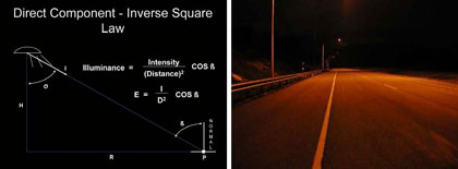
Figure 14 - Inverse Square Law Calculation at a Point
Vertical Illuminance
Vertical illuminance is the amount of illuminance that lands on a vertical surface. The units and properties are the same as horizontal illuminance. As it relates to roadway lighting, vertical illuminance is a reasonable criterion for determining the amount of light landing on pedestrians. It is also used as a criterion in determining adequate illumination for facial recognition. For roadway applications, vertical illuminance is most often used at a 1.5 meter height above the roadway or sidewalk. The 1.5 meter height is a commonly used metric in outdoor criteria as the height of a pedestrian's face.
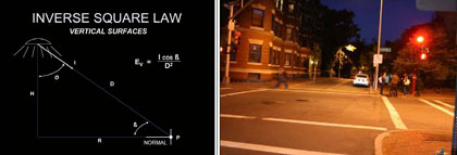
Figure 15 - Calculation of Vertical Illuminance
Luminance
Luminance is the amount of light that reflects from a surface in the direction of the observer. It is often referred to as the "brightness" of the surface, although apparent brightness has a number of other factors to take into consideration. It is, however, a more complete metric than illuminance because it considers not only the amount of light that reaches a surface, but also how much of that light is reflected towards the driver
.
In Figure 16, the roadway has the same illuminance values across both lanes. The luminance values, however, are twice as high for the right lane, which is how the road appears to an observer
Figure 16 - Pavement Reflective Differences
Veiling Luminance Ratio
The veiling luminance ratio is a metric used by the IES and AASHTO to determine the amount of glare generated by a lighting system. The ratio is the maximum veiling luminance at the driver's eye divided by the average pavement luminance of the roadway. Because glare is a function of adaptation luminance, the road is used as the assumed scene from which the luminance reaches the eye.
For example, if a roadway lighting system was designed to a lighting level of 0.6 cd/m2 using 250watt high pressure sodium fixtures of a certain distribution type, the glare would be a certain calculated veiling luminance ratio with the maximum veiling luminance probably being generated from the closest luminaire and the average roadway luminance being 0.6 cd/m2. If the system was changed to use 400 watt lamps, you could expect the veiling luminance to increase by the change in output. But since the scene brightness (roadway luminance) will also increase by the proportional change in output, the veiling luminance ratio or glare of the lighting system will not change.
There are also other metrics which are used to express glare. CIE uses Threshold Increment (TI) as its primary method. TI is based on threshold contrast, which is the amount of contrast between and object and its background when the probability of detection is 50 percent. When glare is introduced, the probability of an object being seen drops below 50 percent, therefore not reaching threshold contrast, which means the contrast needs to be increased. TI is the percentage the contrast needs to be increased in order to achieve threshold contrast again.